Mixed models for quantitative genetics

1/11/2019, OIST

Quantitative genetics

Many traits are quantitative
- Controlled by many genes, each following Mendel’s law
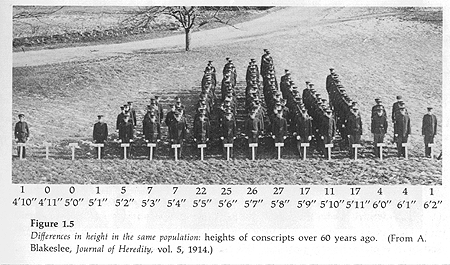
  - They tend to follow a normal distribution
Environment may also play a role
Much of this lecture is based on Wilson et al. (2010)
The tutorial is based on WAMWiki

Partitioning phenotypic variance

\(V_P = V_A + V_R\), where \(V_A\) is the additive genetic variance, and \(V_R\) is the residual (environmental) variance
The narrow-sense heritability of a trait (\(h^{2}\)) is then defined as \(V_p\) explained by \(V_P\) (i.e., \(V_A/V_P\))
- The degree of resemblance between relatives.
For a pair of covarying traits, we can ask whether \(Cov(P)\) is due to additive genetic effects \(Cov(A)\)
- Genetic covariance between traits arises through linkageor pleiotropy
  - It is often expressed as a genetic correlation (\(r_G\))
  - \(r_G\) may constrain phenotypic evolution

A model of an individual’s breeding value

An individual’s ‘breeding value’ is included as an explanatory variable for a phenotypic trait of interest
\[ y_i = \mu + a_i + e_i \]
- \(\mu\) is the population mean
- \(i\) is the individual
- \(a_i\) is the breeding value (the effects of i’s genotype relative to \(\mu\))
However, we don’t know each individual’s breeding value

Mixed-effect models

Random effects models can account for sources of non-independence among data points or avoid pseudoreplication
- Typically, if, say an individual is measured multiple times, it’s id is included as a random effect
- However, random terms allow us to make inferences about the distribution of effects in the population as a whole
  - Including identity as a random effect also yields an estimate of the among-individual variance for \(y\) in the population

Animal model

An animal model is a linear mixed effect model where the breeding value is fitted as a random effect
Data points are not independent, because individuals share genes
By fitting breeding value as a random effect, we obtain an estimate of the additive genetic variance \(V_A\)
In addition we can model variation from other sources (e.g., environmental, sex, etc.)
- e.g., \(y_i = \mu + sex_i + age_i + a_i + e_i\)

Pedigrees to get genetic covariance matrix

Today, these matrixes are often built using genetic data, not pedigrees.

Tutorial: estimating heritability of birth weight

We start with simple model of birth weight in gryphons, using the sommer package, which has the model data set built in

library(sommer)
data(DT_gryphon)
head(DT)

##   ANIMAL MOTHER BYEAR SEX   BWT TARSUS
## 1   1029   1145   968   1 10.77  24.77
## 2   1299    811   968   1  9.30  22.46
## 3    643    642   970   2  3.98  12.89
## 4   1183   1186   970   1  5.39  20.47
## 5   1238   1237   970   2 12.12     NA
## 6    891    895   970   1    NA     NA

dim(A)

## [1] 1309 1309

DT contains animal IDs
A contains the matrix of relatedness

mix1 <- mmer(BWT~1,
             random=~vs(ANIMAL,Gu=A),
             rcov=~units,
             data=DT,
             verbose=FALSE)

summary(mix1)$varcomp

##                   VarComp VarCompSE   Zratio Constraint
## u:ANIMAL.BWT-BWT 3.395393 0.6512306 5.213811   Positive
## units.BWT-BWT    3.828605 0.5309947 7.210251   Positive

ANIMAL.BWT-BWT is the additive variance \(V_A\)
units.BWT-BWT is the residual (unexplained) variance \(V_R\)
Phenotypic variance \(V_P\) is the sum of \(V_A\) and \(V_R\)

Estimating heritability

##                   VarComp
## u:ANIMAL.BWT-BWT 3.395393
## units.BWT-BWT    3.828605

remember \(h^2 = V_A/(V_P) = V_A/(V_A + V_R)\)
\(h^2\) = 3.3953929 / (3.3953929 + 3.8286053) = 0.4700157

Covariance between traits

One of the questions we would like to address is whether traits are independent
This can be done by including multiple traits in the response variable

mix2 <- mmer(cbind(BWT,TARSUS)~1,
             random=~vs(ANIMAL, Gu=A),
             rcov=~vs(units),
             na.method.Y = "include2",
             data=DT, verbose = F)
head(summary(mix2)$varcomp, 3)

##                         VarComp VarCompSE   Zratio Constraint
## u:ANIMAL.BWT-BWT       3.349548 0.6485144 5.164955   Positive
## u:ANIMAL.BWT-TARSUS    1.725953 0.8515828 2.026759   Unconstr
## u:ANIMAL.TARSUS-TARSUS 7.651639 1.9924296 3.840356   Positive

cov2cor(mix2$sigma$`u:ANIMAL`)

##              BWT    TARSUS
## BWT    1.0000000 0.3409248
## TARSUS 0.3409248 1.0000000

Best linear unbiased predictors (BLUPs) of individual breeding values

Mixed models can allow us to solve for individual’s breeding values, which software like sommer report (see docs for the mmer function.
These are assumed to be normally distributed

hist(mix1$U$`u:ANIMAL`$BWT, main = "", xlab = "")

Phylogenetic models are conceptually similar

Species are non-independent, and we can estimate the effect of phylogenetic covariance
We have a adata set and a phylogeny, which from which a covariance matrix is computed

##        phen  cofactor phylo
## 1 107.06595 10.309588  sp_1
## 2  79.61086  9.690507  sp_2
## 3 116.38186 15.007825  sp_3
## 4 143.28705 19.087673  sp_4
## 5 139.60993 15.658404  sp_5

Bayesian model fitting

Here we use brms, which is Bayesian, so we should explicitly specify the priors
The syntax is a bit different, but recognizably similar to what sommer does

model_simple <- brm(
  phen ~ cofactor + (1|phylo), data = data_simple, 
  family = gaussian(), cov_ranef = list(phylo = A),
  prior = c(
    prior(normal(0, 10), "b"),
    prior(normal(0, 50), "Intercept"),
    prior(student_t(3, 0, 20), "sd"),
    prior(student_t(3, 0, 20), "sigma")
  )
)

brms results

summary(model_simple)

##  Family: gaussian 
##   Links: mu = identity; sigma = identity 
## Formula: phen ~ cofactor + (1 | phylo) 
##    Data: data_simple (Number of observations: 200) 
## Samples: 4 chains, each with iter = 2000; warmup = 1000; thin = 1;
##          total post-warmup samples = 4000
## 
## Group-Level Effects: 
## ~phylo (Number of levels: 200) 
##               Estimate Est.Error l-95% CI u-95% CI Eff.Sample Rhat
## sd(Intercept)    14.44      2.20    10.48    19.08        693 1.01
## 
## Population-Level Effects: 
##           Estimate Est.Error l-95% CI u-95% CI Eff.Sample Rhat
## Intercept    38.21      7.07    24.30    52.07       2100 1.00
## cofactor      5.17      0.14     4.91     5.45       6294 1.00
## 
## Family Specific Parameters: 
##       Estimate Est.Error l-95% CI u-95% CI Eff.Sample Rhat
## sigma     9.23      0.74     7.83    10.71       1040 1.01
## 
## Samples were drawn using sampling(NUTS). For each parameter, Eff.Sample 
## is a crude measure of effective sample size, and Rhat is the potential 
## scale reduction factor on split chains (at convergence, Rhat = 1).

Computing phylogenetic signal

This is roughly analagous to \(h^2\) in the animal model

hyp <- "sd_phylo__Intercept^2 / (sd_phylo__Intercept^2 + sigma^2) = 0"
(hyp <- hypothesis(model_simple, hyp, class = NULL))

## Hypothesis Tests for class :
##                 Hypothesis Estimate Est.Error CI.Lower CI.Upper Evid.Ratio
## 1 (sd_phylo__Interc... = 0      0.7      0.09     0.51     0.84         NA
##   Post.Prob Star
## 1        NA    *
## ---
## '*': The expected value under the hypothesis lies outside the 95%-CI.
## Posterior probabilities of point hypotheses assume equal prior probabilities.

plot(hyp)

Other software

As you just saw, there are many ways to actually fit these models, and you are not restricted to one kind of software
While sommer is specifically designed for this type of analysis, basically any package that can fix mixed effects models can be used.
One popular Bayesian option is MCMCglmm, which is relatively fast even for large data sets. However, it is farily non-user friendly, particularly when it comes to setting up priors.
Another option is brms, which is easier to work with, but slower.

Making more complex models

Other matrixes can be included to model more complex processes

Thomson et al. (2018)

Exercises

Make models using (a) sex as a fixed effect (b) year as a random effect and (c) both effects combined.
- How does that change the estimates of heritability? Why do you think this happens?
If you were to breed gryphons for body weight, which would be the best specimen?
Let’s imagine that you didn’t have BWT phenotypes for the first 100 gryphons. Can you still calculate their breeding values?
- Under what circumstances would this be useful?